Getting started

In this page, learn how to use a model developed by somebody else [1]. You can also see how to develop a first model [2] and visualize its outputs [3].

1. Run simulations for an imported project

To import an existing project, see (Documentation / Modelling Platform / Importing a project). If you wish, you can use this one (bellecombe.zip). Once the archive is saved on disk and imported in the OMP, the project appear in the explorer (left window).

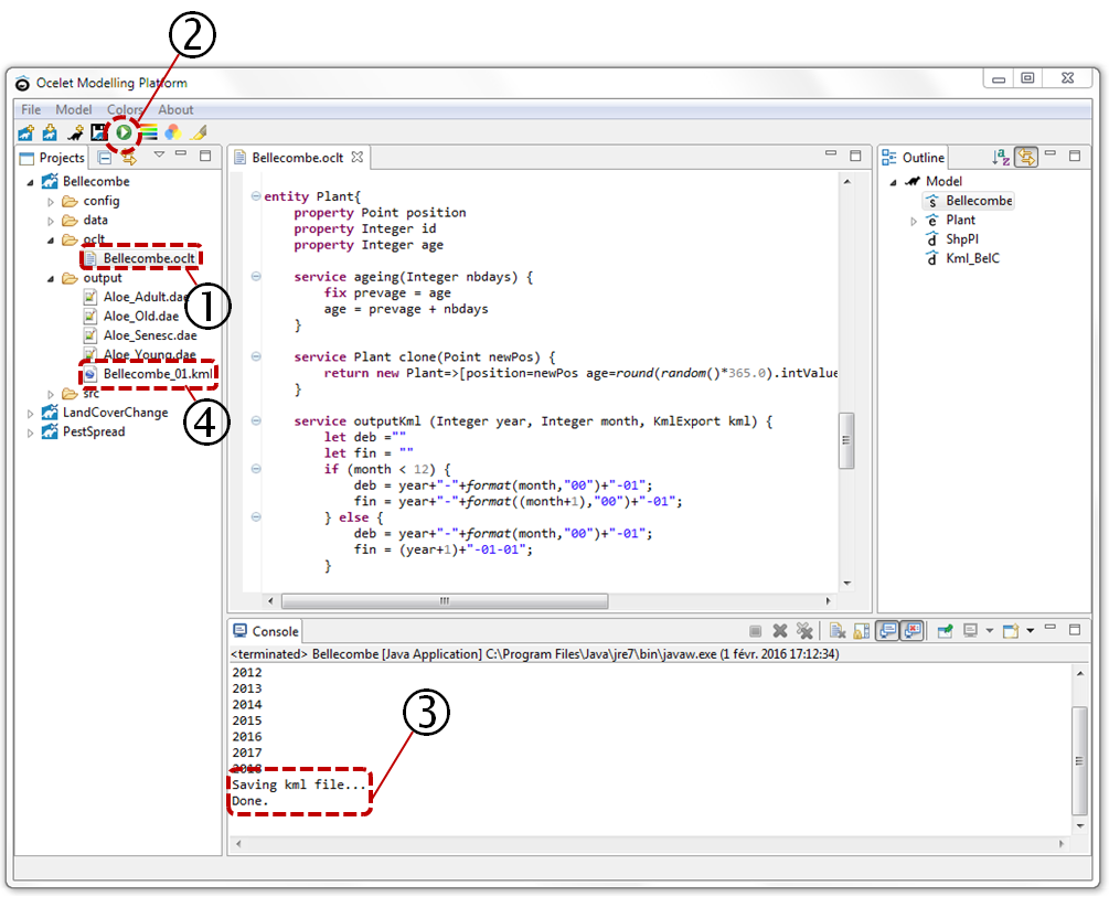
Navigate in the explorer to reach the model "Bellecombe.oclt" (1). When you clic on it, the code of the model appears in the central window, ans its outline in the right one.

To run the simulation (2), clic on .

You can track the simulation in the Console window. Once the end message is displayed (3), the result file appears in the output directory of the project. Refresh project content with F5.

Double-clic on the kml file created (4) to open it in Google Earth.

2. Develop a first model

This little land cover change model is to show how to use some basic functions of Ocelet. As often, we proceed in steps, incrementally. At each intermediate step, the model is incomplete but is able to run.

Create a new project (e.g. Fournaise) with the button. A new subfolder is created in the "workspace" folder. A Shapefile will be needed in "..\workspace\Fournaise\data" and can be obtained after unzipping the following file (AgPlots_Fournaise.zip).

Read entities from a Shapefile and write them in a Kml file

Define the "Agricultural Plot" entity

First, we need to define the entity type used in the model: PlotAg (Agricultural Plot).

This definition is done in the "Fournaise.oclt" file located in "..\workspace\Fournaise\oclt", either before or after (but not inside) the scenario definition:

scenario Fournaise {

    println("Model Fournaise ready to run")

}

// Define the agricultural plot entity. 
entity PlotAg {
    property MultiPolygon geom
    property Integer id
    property Integer lct // land cover type
    property Integer surf // surface area in m²
}

Note that the entity PlotAg has been defined with several property, including one that contains its geometry.

Define the Shapefile and Kml datafacers

Then we need to define how to access the Shapefile from which the PlotAg entities will be read, and also the Kml file into which they will be placed.

// Define a datafacer to read shapefile of plots 
datafacer ShpAg {
    data Shapefile("data/AgPlots_Fournaise.shp","EPSG:32740") // WGS84 UTM40S

    match PlotAg { 
               geom : "geom"
               id : "PID"
               lct : "CCULTURE"
               surf : "SURF"

    }
}

// Define a datafacer for Kml export kml - Land cover
datafacer Kml_LC {
    data KmlExport("output/Fournaise_LandCover.kml")
}

Note that together with the path to the Shapefile, we give an EPSG code that defines the spatial reference system. The match PlotAg part defines how the Shapefile attribute data are read into the property of entities.

Use the entities and the datafacers in a scenario

A service must now be added to the definition of the PlotAg entity so that they can be written in the Kml file,

// Define the agricultural plot entity. 
entity PlotAg {
    property MultiPolygon geom
    property Integer id
    property Integer lct // land cover type
    property Integer surf // surface area in m²

    service outputKml (Integer year, KmlExport kml){
        let id = "Plot" + id + "_" + year
        let style="st" + lct 
        let deb = year+"-01-01"
        let fin = ""+(year+1)+"-01-01"
        kml.addGeometry (style,id, deb, fin, geom, style,0) 

    }
}

and the scenario is modified in order to instantiate the datafacers, read the plot entities from the Shapefile datafacer, define the display styles for the Kml, write in the Kml, and save the Kml.

scenario Fournaise {

    println("Model Fournaise ready to run")

    // Init

    // read Plots from Shapefile  
    let plotShpAg = new ShpAg
    let lplotAg = plotShpAg.readAll()   // returns a list of PlotAg

    // Initialize kml file for output
    let kmln = new Kml_LC
    let plt = colorRange(8,"dem")        // get list of colors from predefined palette "dem"
    kmln.defStyleRange("st",1.0,plt,-0.2) // prefix, line thickness, list of colors , darken line color a little

    // End Init

    // Write land cover state in kml file
    let year = 2014
    for (p:lplotAg) {
          p.outputKml(year, kmln) // write to Kml for each PlotAg of the list
    }               

    // Saving kml file 
    println("")
    println("Saving kml file...")
    kmln.saveAsKml()
    println("Done.")    

}

In "..\workspace\Fournaise\output" you will find the resulting Kml: Fournaise_LandCover.kml

Add a land cover change process and simulate over a period of 10 years

We can now include a land cover change process. Inspired by the Game of Life, the land cover of a plot is modified according to those of neighbouring plots.

Define a neighbourhood relation between plots

The neighbourhood relation defined below contains a filter, an interaction and an aggregation function.

The filter function near with the input parameter dist will keep those edges with a distance between the geometries of plots p1 and p2 less than dist in the condition (p1.geom.distance(p2.geom)< dist. The first condition p1.geom.envelope.distance(p2.geom.envelope) < dist is quicker and will screen out of the test the pairs of geometries whose envelopes are already not close enough.

  relation Neighbourhood<PlotAg p1, PlotAg p2> {
      filter near(Integer dist){
         return (p1.geom.envelope.distance(p2.geom.envelope) < dist) &&
                (p1.geom.distance(p2.geom) < dist)
      }
      interaction changeLC() {
          // the land cover type of a plot is changed according to the lct of its neighbours
          p1.lct =  p2.lct  // a plot receives the lct of the neighbouring plot
          p2.lct =  p1.lct 

      } agg {
          p1.lct << Majority  // a plot has many neighbours, therefore an aggregation function is applied 
          p2.lct << Majority  // default functions (Mean, Min, Max, Sum ...) or user defined (here Majority)
      }
  }

The interaction function changeLC is meant to be applied on each of the edges of the graph. A plot then takes the land cover type lct of its neighbour. As a plot normally has many neighbours, an aggregation function is defined to decide which lct value is assigned to the plot property. Here a user-defined Majority function will choose the most frequent lct among the possible values. But if the selected lct is “too present”, a random value is chosen instead.

The neighbourhood relation can then be used in the scenario. A graph gN is instantiated with all the agricultural plots included but unconnected.

    gN.complete.near(20).connect()

In the above instruction, the near filter is applied to the complete graph, and those agricultural plots that are neighbours less than 20 m apart are connected.

The land cover change function is also applied in the scenario, at each time step, once the states of the agricultural plots are saved in the output files.

    for (year : 2014..2024) {
        println(year)

        // Write land cover state in kml file
        for (p:lplotAg) {
            p.outputKml(year, kmln) // write to Kml for each PlotAg of the list
        }

        // Change land cover according to neighbourhood
        gN.changeLC() 
    }

3. Visualize model outputs

From the scenario above we have seen how the states of the agricultural plots are sent to a kml file at each time step in order to visualize changing land cover types with Google Earth.

Another possibility of displaying animated maps is with QGIS provided the time manager plugin is installed. Time attributes must be added to the agricultural plots before being sent to the output shapefile.

// Define the agricultural plot entity. 
entity PlotAg {
    property MultiPolygon geom
    property Integer id
    property Integer lct // land cover type
    property Integer surf // surface area in m²
    property String date_begin // for use with time manager plugin
    property String date_end  //  in QGIS
}

An output shapefile datafacer can be defined as follows:

datafacer ShpAgOut {
      data Shapefile("output/Fournaise_Landcover.shp","EPSG:32740")
      match PlotAg {
              geom : "the_geom"
              id : "gid"
              lct : "lct"
              date_begin : "begin"
              date_end : "end"
      }
}

In the scenario, the date attributes can be updated and the plots added to a list that will be sent to the output shapefile.

 // simulation
 for (year : 2014..2024) {
    println(year)

    // Initialise list of plots to be added to output shapefile 
    let lplotAgOut = new List<PlotAg>

    // Write land cover state in kml file and shapefile
    for (p:lplotAg) {
        p.outputKml(year, kmln) // write to Kml for each PlotAg of the list

        p.date_begin = ""+ year +"-01-01"
        p.date_end = ""+ year +"-12-31"
        lplotAgOut.add(p)      // add plot to list of plots for shapefile output

    }
    // output to shapefile
    shpout.append(lplotAgOut)

    // Change land cover according to neighbourhood
    gN.changeLC()

 }

At the end, the output shapefile datafacer must be closed for the file to be written on the disk.

 // Saving shapefile  
 print("Saving shp ... ")
 shpout.close()
 println("ok.")

Here is a possible code for the above exercise, and the complete Fournaise model with the corresponding output kml and shapefile.